Progression to Regression: An Introduction to Regression in R
Regression analysis is a powerful statistical tool that allows researchers to investigate relationships between variables, specifically the relationship between a dependent variable and one or more independent variables. In healthcare data, regression analysis is used for numerous purposes:
Prediction and Forecasting: Regression analysis can help forecast future health trends based on historical data. For example, it can predict the prevalence of a disease based on risk factors.
Identifying Risk Factors: Regression analysis can be used to identify risk factors for diseases. For example, it can help determine whether smoking is a significant risk factor for lung cancer.
Cost-effectiveness Analysis: In health economics, regression analysis can help analyze the cost-effectiveness of different treatments or interventions.
Evaluating Treatment Effects: Regression can be used to compare the effects of different treatments in a population, which can inform healthcare decision-making.
Here are some important regression models used in healthcare data analysis:
Linear Regression: Linear regression is used when the dependent variable is continuous. For example, it could be used to examine the relationship between age (independent variable) and blood pressure (dependent variable).
Logistic Regression: Logistic regression is used when the dependent variable is binary, i.e., it has two possible outcomes. It is often used to identify risk factors for diseases. For example, it could be used to investigate the impact of various factors (like age, sex, BMI, smoking status) on the likelihood of developing heart disease (Yes/No).
Cox Regression: Cox regression, or proportional hazards regression, is a type of survival analysis used to investigate the effect of various factors on the time a specified event takes to happen. For example, it can be used to study the survival time of patients after being diagnosed with a certain disease.
Poisson Regression: Poisson regression is used for count data. For instance, it can model the number of hospital admissions over a certain period.
Multilevel Regression: Multilevel (or hierarchical) regression is used when data is grouped, such as patients within hospitals. This takes into account the potential correlation of patients within the same group.
Nonlinear Regression: Nonlinear regression can be used when the relationship between the independent and dependent variables is not linear.
Remember, selecting the appropriate regression model depends largely on the type of data at hand and the specific research question. We will be introducing the approach to univariable and multivariable linear and logistic regression analysis in R.
Before we start lets get some important packages loaded
── Attaching core tidyverse packages ──────────────────────── tidyverse 2.0.0 ──
✔ dplyr     1.1.2     ✔ readr     2.1.4
✔ forcats   1.0.0     ✔ stringr   1.5.0
✔ ggplot2   3.4.2     ✔ tibble    3.2.1
✔ lubridate 1.9.2     ✔ tidyr     1.3.0
✔ purrr     1.0.1
── Conflicts ────────────────────────────────────────── tidyverse_conflicts() ──
✖ dplyr::filter() masks stats::filter()
✖ dplyr::lag()    masks stats::lag()
ℹ Use the conflicted package (<http://conflicted.r-lib.org/>) to force all conflicts to become errors
Loading required package: gtsummary

Loading required package: broom

Loading required package: performance

Loading required package: see

Loading required package: flextable


Attaching package: 'flextable'


The following objects are masked from 'package:gtsummary':

    as_flextable, continuous_summary


The following object is masked from 'package:purrr':

    compose


Loading required package: car

Loading required package: carData


Attaching package: 'car'


The following object is masked from 'package:dplyr':

    recode


The following object is masked from 'package:purrr':

    some
Lets call in the data:
c19_df <-read.csv("https://raw.githubusercontent.com/MoH-Malaysia/covid19-public/main/epidemic/linelist/linelist_deaths.csv")#create a sequence of numbers to represent timec19_df <- c19_df %>%arrange(date) %>%group_by(date) %>%mutate(date_index =cur_group_id(),age_cat=ifelse(age<20, "Less than 20",ifelse(age %in%20:40, "20-40",ifelse(age %in%40:60, "40-60",ifelse(age %in%60:80, "60:80", ">80"))))) %>%ungroup()
Just to be consistent we what I said yesterday- before diving into the data always always skim the data first to get a quick feels
c19_df %>%
  skimr::skim()
Data summary
Name
Piped data
Number of rows
37152
Number of columns
17
_______________________
Column type frequency:
character
11
numeric
6
________________________
Group variables
None
Variable type: character
skim_variable
n_missing
complete_rate
min
max
empty
n_unique
whitespace
date
0
1
10
10
0
1004
0
date_announced
0
1
10
10
0
1000
0
date_positive
0
1
10
10
0
999
0
date_dose1
0
1
0
10
22437
298
0
date_dose2
0
1
0
10
28034
267
0
date_dose3
0
1
0
10
35719
161
0
brand1
0
1
0
16
22437
8
0
brand2
0
1
0
16
28034
7
0
brand3
0
1
0
16
35719
6
0
state
0
1
5
17
0
16
0
age_cat
0
1
3
12
0
5
0
Variable type: numeric
skim_variable
n_missing
complete_rate
mean
sd
p0
p25
p50
p75
p100
hist
age
0
1
62.65
16.59
0
51
64
75
130
▁▃▇▃▁
male
0
1
0.58
0.49
0
0
1
1
1
▆▁▁▁▇
bid
0
1
0.21
0.41
0
0
0
0
1
▇▁▁▁▂
malaysian
0
1
0.89
0.31
0
1
1
1
1
▁▁▁▁▇
comorb
0
1
0.79
0.41
0
1
1
1
1
▂▁▁▁▇
date_index
0
1
419.07
122.14
1
362
393
444
1004
▁▇▆▁▁
Linear regression
The R function lm() perform linear regression, assessing the relationship between numeric response and explanatory variables that are assumed to have a linear relationship.
Provide the equation as a formula, with the response and explanatory column names separated by a tilde ~. Also, specify the dataset to data =. Define the model results as an R object, to use later.
Univariate linear regression
lm_results <-lm(age ~ malaysian, data = c19_df)
You can then run summary() on the model results to see the coefficients (Estimates), P-value, residuals, and other measures.
summary(lm_results)
Call:
lm(formula = age ~ malaysian, data = c19_df)

Residuals:
   Min     1Q Median     3Q    Max
-64.26 -10.26   0.74  11.74  80.53

Coefficients:
            Estimate Std. Error t value Pr(>|t|)
(Intercept)  49.4727     0.2509  197.14   <2e-16 ***
malaysian    14.7875     0.2658   55.63   <2e-16 ***
---
Signif. codes:  0 '***' 0.001 '**' 0.01 '*' 0.05 '.' 0.1 ' ' 1

Residual standard error: 15.94 on 37150 degrees of freedom
Multiple R-squared:  0.07691,   Adjusted R-squared:  0.07689
F-statistic:  3095 on 1 and 37150 DF,  p-value: < 2.2e-16
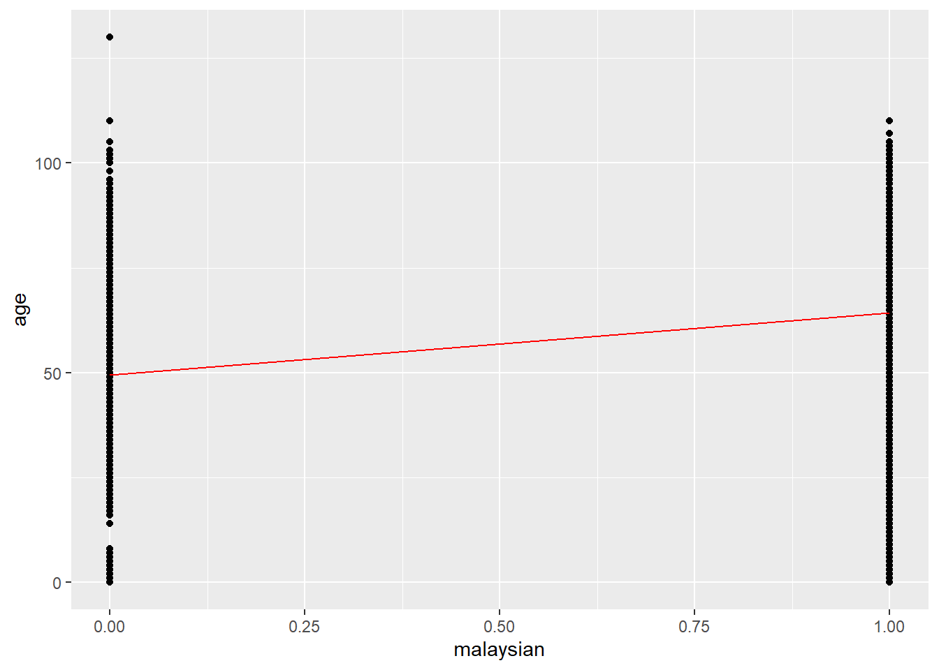
Alternatively you can use the tidy() function from the broom package to pull the results in to a table. What the results tell us is that Malaysians (change from 0 to 1) the age of COVID-19 death increases by 14.8 years and this is statistically significant (p<0.01).
You can then also use this regression to add it to a ggplot, to do this we first pull the points for the observed data and the fitted line in to one data frame using the augment() function from broom.
## pull the regression points and observed data in to one datasetpoints <-augment(lm_results)## plot the data using age as the x-axis ggplot(points, aes(x = malaysian)) +## add points for height geom_point(aes(y = age)) +## add your regression line geom_line(aes(y = .fitted), colour ="red")
Note
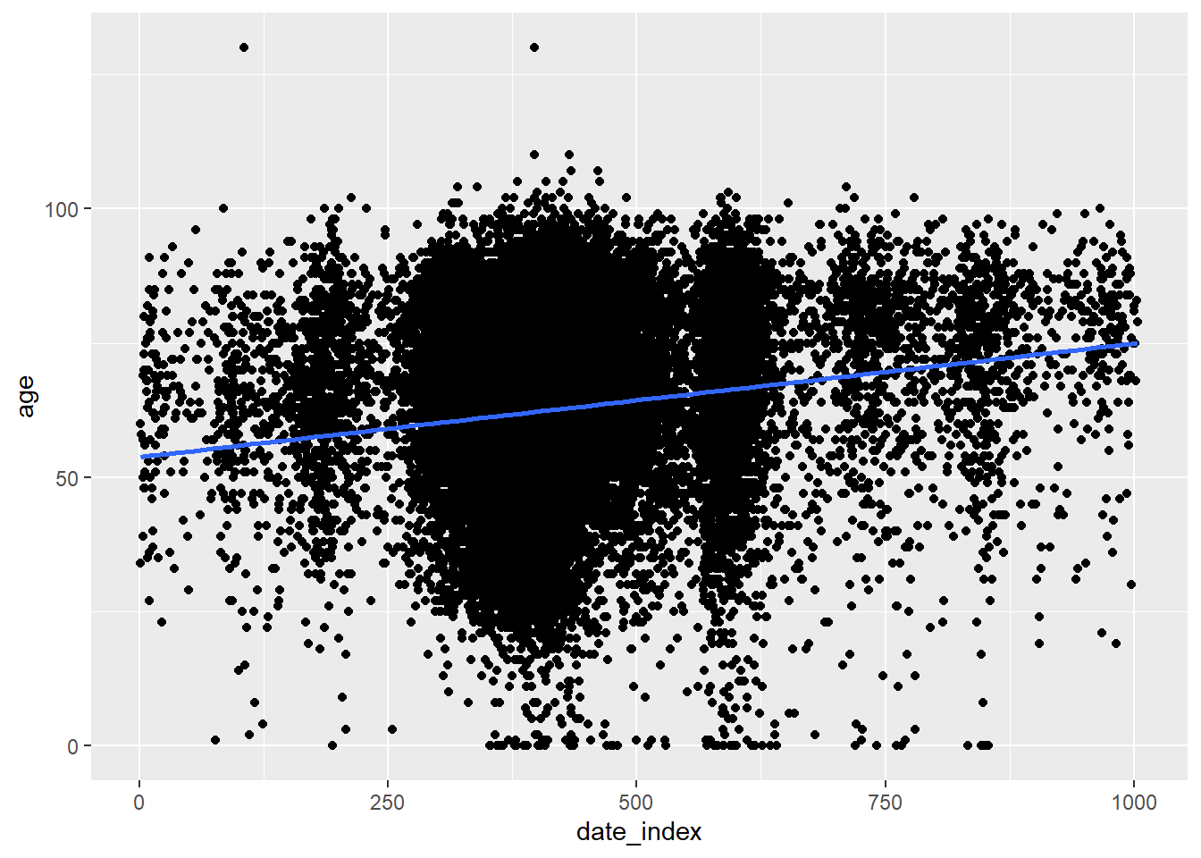
When using a categorical variable as the predictor as we did above the plots can appear somewhat difficult to understand. We can try using a continuous on continuous method and implement it more simpler directly in ggplot and it should look like:
## add your data to a plot ggplot(c19_df, aes(x = date_index, y = age)) +## show pointsgeom_point() +## add a linear regression geom_smooth(method ="lm", se =FALSE)
`geom_smooth()` using formula = 'y ~ x'
Multivariable linear regression
There is almost no difference when carrying out multivariable linear regression, instead we just add on the expression + to add more variables to the equation.
lm_results <-lm(age ~ malaysian + bid + male + state + comorb, data = c19_df)
The function glm() from the stats package (part of base R) is used to fit Generalized Linear Models (GLM). glm() can be used for univariate and multivariable logistic regression (e.g. to get Odds Ratios). Here are the core parts:
formula = The model is provided to glm() as an equation, with the outcome on the left and explanatory variables on the right of a tilde ~.
family = This determines the type of model to run. For logistic regression, use family = "binomial", for poisson use family = "poisson". Other examples are in the table below.
data = Specify your data frame
If necessary, you can also specify the link function via the syntax family = familytype(link = "linkfunction")). You can read more in the documentation about other families and optional arguments such as weights = and subset = (?glm).
Family
Default link function
"binomial"
(link = "logit")
"gaussian"
(link = "identity")
"Gamma"
(link = "inverse")
"inverse.gaussian"
(link = "1/mu^2")
"poisson"
(link = "log")
"quasi"
(link = "identity", variance = "constant")
"quasibinomial"
(link = "logit")
"quasipoisson"
(link = "log")
When running glm() it is most common to save the results as a named R object. Then you can print the results to your console using summary() as shown below, or perform other operations on the results (e.g. exponentiate). If you need to run a negative binomial regression you can use the MASS package; the glm.nb() uses the same syntax as glm(). For a walk-through of different regressions, see the UCLA stats page. So lets try to run a logistic regression model first:
model <-glm(malaysian ~ age_cat, family ="binomial", data = c19_df)summary(model)
Call:
glm(formula = malaysian ~ age_cat, family = "binomial", data = c19_df)

Deviance Residuals:
    Min       1Q   Median       3Q      Max
-2.7224   0.2231   0.2747   0.6605   0.7777

Coefficients:
                    Estimate Std. Error z value Pr(>|z|)
(Intercept)          3.68075    0.08588  42.859  < 2e-16 ***
age_cat20-40        -2.63967    0.09382 -28.135  < 2e-16 ***
age_cat40-60        -2.26931    0.08895 -25.512  < 2e-16 ***
age_cat60:80        -0.42226    0.09566  -4.414 1.01e-05 ***
age_catLess than 20 -2.19915    0.18614 -11.814  < 2e-16 ***
---
Signif. codes:  0 '***' 0.001 '**' 0.01 '*' 0.05 '.' 0.1 ' ' 1

(Dispersion parameter for binomial family taken to be 1)

    Null deviance: 25526  on 37151  degrees of freedom
Residual deviance: 22412  on 37147  degrees of freedom
AIC: 22422

Number of Fisher Scoring iterations: 6
Can you spot a potential issue in the summary above?
c19_df %>%mutate(age_cat =fct_relevel(age_cat, "Less than 20", after =0)) %>%glm(formula = malaysian ~ age_cat, family ="binomial") %>%summary()
Call:
glm(formula = malaysian ~ age_cat, family = "binomial", data = .)

Deviance Residuals:
    Min       1Q   Median       3Q      Max
-2.7224   0.2231   0.2747   0.6605   0.7777

Coefficients:
             Estimate Std. Error z value Pr(>|z|)
(Intercept)   1.48160    0.16514   8.972  < 2e-16 ***
age_cat>80    2.19915    0.18614  11.814  < 2e-16 ***
age_cat20-40 -0.44052    0.16941  -2.600  0.00931 **
age_cat40-60 -0.07017    0.16676  -0.421  0.67394
age_cat60:80  1.77689    0.17043  10.426  < 2e-16 ***
---
Signif. codes:  0 '***' 0.001 '**' 0.01 '*' 0.05 '.' 0.1 ' ' 1

(Dispersion parameter for binomial family taken to be 1)

    Null deviance: 25526  on 37151  degrees of freedom
Residual deviance: 22412  on 37147  degrees of freedom
AIC: 22422

Number of Fisher Scoring iterations: 6
Lets clean that up so we have a nice exponentiated and round up the hyper precise output:
model <-glm(malaysian ~ age_cat, family ="binomial", data = c19_df) %>%tidy(exponentiate =TRUE, conf.int =TRUE) %>%# exponentiate and produce CIsmutate(across(where(is.numeric), round, digits =2)) # round all numeric columns
Warning: There was 1 warning in `mutate()`.
ℹ In argument: `across(where(is.numeric), round, digits = 2)`.
Caused by warning:
! The `...` argument of `across()` is deprecated as of dplyr 1.1.0.
Supply arguments directly to `.fns` through an anonymous function instead.

  # Previously
  across(a:b, mean, na.rm = TRUE)

  # Now
  across(a:b, \(x) mean(x, na.rm = TRUE))
If you want to include two variables and an interaction between them you can separate them with an asterisk * instead of a +. Separate them with a colon : if you are only specifying the interaction. For example:
log_intrx_reg <-glm(malaysian ~ age_cat*bid + comorb + male + state, family ="binomial", data = c19_df)tidy(log_reg, exponentiate =TRUE, conf.int =TRUE)
You can build your model step-by-step, saving various models that include certain explanatory variables. You can compare these models with likelihood-ratio tests using lrtest() from the package lmtest, as below:
model1 <-glm(malaysian ~ age_cat, family ="binomial", data = c19_df)model2 <-glm(malaysian ~ age_cat + bid, family ="binomial", data = c19_df)lmtest::lrtest(model1, model2)
If you prefer to instead leverage the computation available within you processor we can instead take the model object and apply the step() function from the stats package. Specify which variable selection direction you want use when building the model.
## choose a model using forward selection based on AIC## you can also do "backward" or "both" by adjusting the directionfinal_log_reg <- log_reg %>%step(direction ="both", trace =FALSE)
Check the best fitting models based on both a backward and forward method
log_tab_base <- final_log_reg %>% broom::tidy(exponentiate =TRUE, conf.int =TRUE) %>%## get a tidy dataframe of estimates mutate(across(where(is.numeric), round, digits =2)) ## round #checklog_tab_base
My favourite package again. The gtsummary package provides the tbl_regression() function, which will take the outputs from a regression (glm() in this case) and produce an nice summary table.
## show results table of final regression mv_tab <-tbl_regression(final_log_reg, exponentiate =TRUE)#checkmv_tab
Characteristic
OR1
95% CI1
p-value
age_cat
>80
—
—
20-40
0.07
0.06, 0.09
<0.001
40-60
0.11
0.09, 0.13
<0.001
60:80
0.53
0.44, 0.65
<0.001
Less than 20
0.14
0.10, 0.21
<0.001
bid
0.28
0.26, 0.31
<0.001
comorb
3.45
3.20, 3.73
<0.001
male
1.09
1.01, 1.18
0.022
state
Johor
—
—
Kedah
3.37
2.58, 4.45
<0.001
Kelantan
2.75
1.91, 4.09
<0.001
Melaka
2.22
1.61, 3.14
<0.001
Negeri Sembilan
1.30
1.00, 1.71
0.055
Pahang
1.86
1.33, 2.65
<0.001
Perak
2.85
2.11, 3.92
<0.001
Perlis
2.75
1.10, 9.25
0.057
Pulau Pinang
0.81
0.66, 1.00
0.044
Sabah
0.26
0.23, 0.31
<0.001
Sarawak
4.49
2.96, 7.15
<0.001
Selangor
0.47
0.41, 0.54
<0.001
Terengganu
3.16
1.96, 5.44
<0.001
W.P. Kuala Lumpur
0.40
0.34, 0.47
<0.001
W.P. Labuan
0.44
0.28, 0.72
<0.001
W.P. Putrajaya
34,834
340, 10,238,707,683,122,566
>0.9
1 OR = Odds Ratio, CI = Confidence Interval
Its so good! But it doesn’t end there. tbl_uvregression() from the gtsummary package produces a table of univariate regression results. We select only the necessary columns from the linelist (explanatory variables and the outcome variable) and pipe them into tbl_uvregression(). We are going to run univariate regression on each of the columns we defined as explanatory_vars in the data
Within the function itself, we provide the method = as glm (no quotes), the y = outcome column (outcome), specify to method.args = that we want to run logistic regression via family = binomial, and we tell it to exponentiate the results.
The output is HTML and contains the counts
## define variables of interest explanatory_vars <-c("bid", "male", "comorb", "age_cat", "state")#lets leave state ut to increase the computation#cteate a data subset and run the regressionuniv_tab <- c19_df %>% dplyr::select(explanatory_vars, malaysian) %>%## select variables of interesttbl_uvregression( ## produce univariate tablemethod = glm, ## define regression want to run (generalised linear model)y = malaysian, ## define outcome variablemethod.args =list(family = binomial), ## define what type of glm want to run (logistic)exponentiate =TRUE## exponentiate to produce odds ratios (rather than log odds) )## view univariate results table univ_tab
Characteristic
N
OR1
95% CI1
p-value
bid
37,152
0.20
0.19, 0.22
<0.001
male
37,152
0.93
0.87, 0.99
0.029
comorb
37,152
5.61
5.24, 6.00
<0.001
age_cat
37,152
>80
—
—
20-40
0.07
0.06, 0.09
<0.001
40-60
0.10
0.09, 0.12
<0.001
60:80
0.66
0.54, 0.79
<0.001
Less than 20
0.11
0.08, 0.16
<0.001
state
37,152
Johor
—
—
Kedah
3.21
2.49, 4.20
<0.001
Kelantan
3.65
2.57, 5.37
<0.001
Melaka
2.22
1.63, 3.10
<0.001
Negeri Sembilan
1.51
1.19, 1.95
0.001
Pahang
1.98
1.45, 2.79
<0.001
Perak
3.40
2.55, 4.61
<0.001
Perlis
4.08
1.72, 13.3
0.006
Pulau Pinang
0.85
0.71, 1.03
0.094
Sabah
0.34
0.29, 0.38
<0.001
Sarawak
6.45
4.32, 10.1
<0.001
Selangor
0.41
0.36, 0.46
<0.001
Terengganu
4.37
2.76, 7.43
<0.001
W.P. Kuala Lumpur
0.33
0.29, 0.38
<0.001
W.P. Labuan
0.39
0.26, 0.61
<0.001
W.P. Putrajaya
65,203
434, 166,983,382,533,055,616
>0.9
1 OR = Odds Ratio, CI = Confidence Interval
Now for some magic
## combine with univariate results mv_merge <-tbl_merge(tbls =list(univ_tab, mv_tab), # combinetab_spanner =c("**Univariate**", "**Multivariable**")) # set header names#checkmv_merge
Characteristic
Univariate
Multivariable
N
OR1
95% CI1
p-value
OR1
95% CI1
p-value
bid
37,152
0.20
0.19, 0.22
<0.001
0.28
0.26, 0.31
<0.001
male
37,152
0.93
0.87, 0.99
0.029
1.09
1.01, 1.18
0.022
comorb
37,152
5.61
5.24, 6.00
<0.001
3.45
3.20, 3.73
<0.001
age_cat
37,152
>80
—
—
—
—
20-40
0.07
0.06, 0.09
<0.001
0.07
0.06, 0.09
<0.001
40-60
0.10
0.09, 0.12
<0.001
0.11
0.09, 0.13
<0.001
60:80
0.66
0.54, 0.79
<0.001
0.53
0.44, 0.65
<0.001
Less than 20
0.11
0.08, 0.16
<0.001
0.14
0.10, 0.21
<0.001
state
37,152
Johor
—
—
—
—
Kedah
3.21
2.49, 4.20
<0.001
3.37
2.58, 4.45
<0.001
Kelantan
3.65
2.57, 5.37
<0.001
2.75
1.91, 4.09
<0.001
Melaka
2.22
1.63, 3.10
<0.001
2.22
1.61, 3.14
<0.001
Negeri Sembilan
1.51
1.19, 1.95
0.001
1.30
1.00, 1.71
0.055
Pahang
1.98
1.45, 2.79
<0.001
1.86
1.33, 2.65
<0.001
Perak
3.40
2.55, 4.61
<0.001
2.85
2.11, 3.92
<0.001
Perlis
4.08
1.72, 13.3
0.006
2.75
1.10, 9.25
0.057
Pulau Pinang
0.85
0.71, 1.03
0.094
0.81
0.66, 1.00
0.044
Sabah
0.34
0.29, 0.38
<0.001
0.26
0.23, 0.31
<0.001
Sarawak
6.45
4.32, 10.1
<0.001
4.49
2.96, 7.15
<0.001
Selangor
0.41
0.36, 0.46
<0.001
0.47
0.41, 0.54
<0.001
Terengganu
4.37
2.76, 7.43
<0.001
3.16
1.96, 5.44
<0.001
W.P. Kuala Lumpur
0.33
0.29, 0.38
<0.001
0.40
0.34, 0.47
<0.001
W.P. Labuan
0.39
0.26, 0.61
<0.001
0.44
0.28, 0.72
<0.001
W.P. Putrajaya
65,203
434, 166,983,382,533,055,616
>0.9
34,834
340, 10,238,707,683,122,566
>0.9
1 OR = Odds Ratio, CI = Confidence Interval
One final piece of magic! We can export our publication ready regression table into a document. Lovely!
Model evaluation in r using the performance() and car()
Lets just run through quickly how we can evaluate linear and logistics models in R.
Linear model evaluation
Linearity and Homoscedasticity: These can be checked using a residuals vs fitted values plot.
For linearity, we expect to see no pattern or curve in the points, while for homoscedasticity, we expect the spread of residuals to be approximately constant across all levels of the independent variables.
check_model(lm_results)
Normality of residuals: This can be checked using a QQ plot.
If the residuals are normally distributed, the points in the QQ plot will generally follow the straight line.
check_normality(model)
Independence of residuals (No autocorrelation): This can be checked using the Durbin-Watson test.
If the test statistic is approximately 2, it indicates no autocorrelation.
check_autocorrelation(model)
No multicollinearity: This can be checked using Variance Inflation Factor (VIF).
A VIF value greater than 5 (some suggest 10) might indicate problematic multicollinearity.
check_collinearity(model)
Logistic model evaluation
Binary Outcome: Logistic regression requires the dependent variable to be binary or ordinal in ordinal logistic regression.
Observation Independence: Observations should be independent of each other. This is more of a study design issue than something you would check with a statistical test.
No Multicollinearity: Just like in linear regression, the independent variables should not be highly correlated with each other.
Just like in linear regression, a rule of thumb is that if the VIF is greater than 5 (or sometimes 10), then the multicollinearity is high.
# Checking for Multicollinearity:check_collinearity(mv_model)
Linearity of Log Odds: While logistic regression does not assume linearity of the relationship between the independent variables and the dependent variable, it does assume linearity of independent variables and the log odds.
Checking for Linearity of Log Odds:
Logistic regression assumes that the log odds of the outcome is a linear combination of the independent variables. This is a complex assumption to check, but one approach is to look for significant interactions between your predictors and the log odds.
First, fit a model that allows for the possibility of a non-linear relationship:
If the model with the quadratic term is significantly better than the model without (i.e., p < 0.05), this could be a sign that the assumption of linearity of the log odds has been violated.
Acknowledgements
Material for this lecture was borrowed and adopted from