Untangling Data with Tidyverse: Data wranggling in R
Data cleaning is arguably the most crucial step in the data analysis pipeline because it directly impacts the accuracy and reliability of insights drawn from the data.
Garbage in, garbage out, as the saying goes.
Without thoroughly cleaning the data, we might be working with incorrect, inconsistent, or irrelevant information, leading to potentially faulty conclusions. Data cleaning ensures the data is correctly formatted, accurate, complete, and ready for analysis. It involves dealing with missing values, removing duplicates, correcting inconsistencies, and handling outliers. Only after a rigorous data cleaning process can we trust that our analysis or model will give us meaningful, actionable insights.
Thus, while it can be a time-consuming process, skipping or skimping on data cleaning can lead to wasting even more time and resources downstream, as we try to interpret misleading results or troubleshoot models that aren’t performing as expected.
The “Tidyverse”
There are a number of R packages that take advantage of the tidy data form and can be used to do interesting things with data. Many (but not all) of these packages are written by Hadley Wickham and the collection of packages is often referred to as the “tidyverse” because of their dependence on and presumption of tidy data.
A subset of the “Tidyverse” packages include:
ggplot2: a plotting system based on the grammar of graphics
magrittr: defines the %>% operator for chaining functions together in a series of operations on data
dplyr: a suite of (fast) functions for working with data frames
tidyr: easily tidy data with pivot_wider() and pivot_longer() functions (also separate() and unite())
We can call in the tidyverse as mentioned in the introduction like this:
library(tidyverse)
Warning: package 'tidyverse' was built under R version 4.2.3
Warning: package 'ggplot2' was built under R version 4.2.3
Warning: package 'tibble' was built under R version 4.2.3
Warning: package 'tidyr' was built under R version 4.2.3
Warning: package 'readr' was built under R version 4.2.3
Warning: package 'purrr' was built under R version 4.2.3
Warning: package 'dplyr' was built under R version 4.2.3
Warning: package 'stringr' was built under R version 4.2.3
Warning: package 'forcats' was built under R version 4.2.3
Warning: package 'lubridate' was built under R version 4.2.3
── Attaching core tidyverse packages ──────────────────────── tidyverse 2.0.0 ──
✔ dplyr     1.1.2     ✔ readr     2.1.4
✔ forcats   1.0.0     ✔ stringr   1.5.0
✔ ggplot2   3.4.2     ✔ tibble    3.2.1
✔ lubridate 1.9.2     ✔ tidyr     1.3.0
✔ purrr     1.0.1
── Conflicts ────────────────────────────────────────── tidyverse_conflicts() ──
✖ dplyr::filter() masks stats::filter()
✖ dplyr::lag()    masks stats::lag()
ℹ Use the conflicted package (<http://conflicted.r-lib.org/>) to force all conflicts to become errors
Data Frames
The data frame (or data.frame) is a key data structure in statistics and in R.
The basic structure of a data frame is that there is one observation per row and each column represents a variable, a measure, feature, or characteristic of that observation.
Tibbles
Another type of data structure that we need to discuss is called the tibble! It’s best to think of tibbles as an updated and stylish version of the data.frame.
Before we go any further, tibbles are data frames, but they have some new bells and whistles to make your life easier.
How tibbles differ from data.frame
Input type remains unchanged - data.frame is notorious for treating strings as factors; this will not happen with tibbles
Variable names remain unchanged - In base R, creating data.frames will remove spaces from names, converting them to periods or add “x” before numeric column names. Creating tibbles will not change variable (column) names.
There are no row.names() for a tibble - Tidy data requires that variables be stored in a consistent way, removing the need for row names.
Tibbles print first ten rows and columns that fit on one screen - Printing a tibble to screen will never print the entire huge data frame out. By default, it just shows what fits to your screen.
Converting to data.frame or tibble
Use the as.data.frame() or as_tibble()
Calling in some data
For the purposes of this session lets utilise the Malaysian COVID-19 deaths linelinest maintained by the Ministry of Health on their Github page. Codes for each column are as follows:
date: yyyy-mm-dd format; date of death
date_announced: date on which the death was announced to the public (i.e. registered in the public linelist)
date_positive: date of positive sample
date_doseN: date of the individual’s first/second/third dose (if any)
brandN: p = Pfizer, s = Sinovac, a = AstraZeneca, c = Cansino, m = Moderna, h = Sinopharm, j = Janssen, u = unverified (pending sync with VMS)
state: state of residence
age: age as an integer; note that it is possible for age to be 0, denoting infants less than 6 months old
male: binary variable with 1 denoting male and 0 denoting female
bid: binary variable with 1 denoting brought-in-dead and 0 denoting an inpatient death
malaysian: binary variable with 1 denoting Malaysian and 0 denoting non-Malaysian
comorb: binary variable with 1 denoting that the individual has comorbidities and 0 denoting no comorbidities declared
The dplyr package was developed by Posit (formely RStudio) and is an optimized and distilled version of the older plyrpackage for data manipulation or wrangling.
The dplyr package does not provide any “new” functionality to R per se, in the sense that everything dplyr does could already be done with base R, but it greatly simplifies existing functionality in R.
One important contribution of the dplyr package is that it provides a “grammar” (in particular, verbs) for data manipulation and for operating on data frames.
With this grammar, you can sensibly communicate what it is that you are doing to a data frame that other people can understand (assuming they also know the grammar). This is useful because it provides an abstraction for data manipulation that previously did not exist.
Another useful contribution is that the dplyr functions are very fast, as many key operations are coded in C++.
dplyr grammar
Some of the key “verbs” provided by the dplyr package are
select(): return a subset of the columns of a data frame, using a flexible notation
filter(): extract a subset of rows from a data frame based on logical conditions
arrange(): reorder rows of a data frame
rename(): rename variables in a data frame
mutate(): add new variables/columns or transform existing variables
summarise() / summarize(): generate summary statistics of different variables in the data frame, possibly within strata
%>%: the “pipe” operator is used to connect multiple verb actions together into a pipelineArtwork by
select()
Lets convert the COVID-19 deaths linelist into a tibble first
# A tibble: 6 × 6
  state     age  male   bid malaysian comorb
  <chr>   <int> <int> <int>     <int>  <int>
1 Johor      34     1     0         1      1
2 Sarawak    60     1     0         1      1
3 Sabah      58     1     0         1      1
4 Melaka     50     1     0         1      1
5 Sarawak    80     0     1         1      1
6 Sarawak    39     0     0         1      1
Note
The : normally cannot be used with names or strings, but inside the select() function you can use it to specify a range of variable names.
You can also omit variables using the select() function by using the negative sign. With select() you can do
select(c19_df, -(state:comorb))
The select() function also allows a special syntax that allows you to specify variable names based on patterns. So, for example, if you wanted to keep every variable that ends with a “2”, we could do
You can also use more general regular expressions if necessary. See the help page (?select) for more details.
filter()
The filter() function is used to extract subsets of rows from a data frame. This function is similar to the existing subset() function in R but is quite a bit faster in my experience.
You can see that there are now only 22276 rows in the data frame and the distribution of the age values is.
summary(c19_filter$age)
   Min. 1st Qu.  Median    Mean 3rd Qu.    Max.
   60.0    66.0    73.0    73.7    81.0   130.0
We can place an arbitrarily complex logical sequence inside of filter(), so we could for example extract the rows where age is greater than 60 and nationality (malaysian) is equal to 1
c19_filter <-filter(c19_df, age <21& malaysian==1)select(c19_filter, date, malaysian, age)
Now there are only 221 observations where both of those conditions are met.
Other logical operators you should be aware of include:
Operator
Meaning
Example
==
Equals
malaysian== 1
!=
Does not equal
malaysian!= 1
>
Greater than
age> 60
>=
Greater than or equal to
age>= 60
<
Less than
age< 60
<=
Less than or equal to
age<= 60
%in%
Included in
state %in% c("Selangor", "Johor")
is.na()
Is a missing value
is.na(date_dose_2)
Note
If you are ever unsure of how to write a logical statement, but know how to write its opposite, you can use the ! operator to negate the whole statement.
A common use of this is to identify observations with non-missing data (e.g., !(is.na(date_dose_2))).
arrange()
The arrange() function is used to reorder rows of a data frame according to one of the variables/columns. Reordering rows of a data frame (while preserving corresponding order of other columns) is normally a pain to do in R. The arrange() function simplifies the process quite a bit.
Here we can order the rows of the data frame by date, so that the first row is the earliest (oldest) observation and the last row is the latest (most recent) observation.
c19_df <-arrange(c19_df, date)
We can now check the first few rows
head(select(c19_df, date, age), 3)
# A tibble: 3 × 2
  date         age
  <chr>      <int>
1 2020-03-17    34
2 2020-03-17    60
3 2020-03-20    58
Columns can be arranged in descending order too by useing the special desc() operator.
c19_df <-arrange(c19_df, desc(date))
Looking at the first three and last three rows shows the dates in descending order.
head(select(c19_df, date, age), 3)
# A tibble: 3 × 2
  date         age
  <chr>      <int>
1 2023-06-27    79
2 2023-06-26    83
3 2023-06-22    68
tail(select(c19_df, date, age), 3)
# A tibble: 3 × 2
  date         age
  <chr>      <int>
1 2020-03-20    58
2 2020-03-17    34
3 2020-03-17    60
rename()
Renaming a variable in a data frame in R is surprisingly hard to do! The rename() function is designed to make this process easier.
Here you can see the names of the first six variables in the c19_df data frame.
These names are (arbitrarily again) unnecessarily long. Date doesn’t need to be repeated for each column name are no other columns that could potentially be confused with the first six. So we can modify cause we’re lazy to type long column names when analysing later on.
The syntax inside the rename() function is to have the new name on the left-hand side of the = sign and the old name on the right-hand side.
mutate()
The mutate() function exists to compute transformations of variables in a data frame. Often, you want to create new variables that are derived from existing variables and mutate() provides a clean interface for doing that.
Warning: There was 1 warning in `mutate()`.
ℹ In argument: `brand2 = recode(...)`.
Caused by warning:
! Unreplaced values treated as NA as `.x` is not compatible.
Please specify replacements exhaustively or supply `.default`.
group_by()
The group_by() function is used to generate summary statistics from the data frame within strata defined by a variable.
For example, in this dataset, you might want to know what the number of deaths in each state is?
In conjunction with the group_by() function, we often use the summarise() function
Note
The general operation here is a combination of
Splitting a data frame into separate pieces defined by a variable or group of variables (group_by())
Then, applying a summary function across those subsets (summarise())
Example
We can create a separate data frame that splits the original data frame by state
state <-group_by(c19_df, state)
We can then compute summary statistics for each year in the data frame with the summarise() function.
summarise(state, age =mean(age, na.rm =TRUE),age_median=median(age, na.rm =TRUE))
# A tibble: 16 × 3
   state               age age_median
   <chr>             <dbl>      <dbl>
 1 Johor              60.9       60.9
 2 Kedah              63.1       63.1
 3 Kelantan           66.7       66.7
 4 Melaka             62.2       62.2
 5 Negeri Sembilan    64.5       64.5
 6 Pahang             63.2       63.2
 7 Perak              66.9       66.9
 8 Perlis             68.1       68.1
 9 Pulau Pinang       66.0       66.0
10 Sabah              65.4       65.4
11 Sarawak            68.1       68.1
12 Selangor           59.4       59.4
13 Terengganu         64.9       64.9
14 W.P. Kuala Lumpur  61.7       61.7
15 W.P. Labuan        59.3       59.3
16 W.P. Putrajaya     64.7       64.7
%>%
The pipeline operator %>% is very handy for stringing together multiple dplyr functions in a sequence of operations.
Notice above that every time we wanted to apply more than one function, the sequence gets buried in a sequence of nested function calls that is difficult to read, i.e. This nesting is not a natural way to think about a sequence of operations.
The %>% operator allows you to string operations in a left-to-right fashion, i.e
Example
Take the example that we just did in the last section.
That can be done with the following sequence in a single R expression.
`summarise()` has grouped output by 'state'. You can override using the
`.groups` argument.
# A tibble: 46 × 4
# Groups:   state [16]
   state    age_cat   age age_median
   <chr>    <chr>   <dbl>      <dbl>
 1 Johor    20-59   45.8       45.8
 2 Johor    <19      8.62       8.62
 3 Johor    >60     73.5       73.5
 4 Kedah    20-59   46.9       46.9
 5 Kedah    <19      7.47       7.47
 6 Kedah    >60     73.7       73.7
 7 Kelantan 20-59   47.7       47.7
 8 Kelantan <19     14.4       14.4
 9 Kelantan >60     74.1       74.1
10 Melaka   20-59   46.0       46.0
# ℹ 36 more rows
This way we do not have to create a set of temporary variables along the way or create a massive nested sequence of function calls.
slice_*()
The slice_sample() function of the dplyr package will allow you to see a sample of random rows in random order.
The number of rows to show is specified by the n argument.
This can be useful if you do not want to print the entire tibble, but you want to get a greater sense of the values.
This is a good option for data analysis reports, where printing the entire tibble would not be appropriate if the tibble is quite large.
Example
slice_sample(c19_df, n =10)
# A tibble: 10 × 16
   death   announced positive dose1 dose2 dose3 brand1 brand2 brand3 state   age
   <chr>   <chr>     <chr>    <chr> <chr> <chr> <chr>   <dbl> <chr>  <chr> <int>
 1 2021-0… 2021-09-… 2021-08… ""    ""    ""    ""         NA ""     Kedah    58
 2 2021-0… 2021-08-… 2021-08… ""    ""    ""    ""         NA ""     Johor    63
 3 2022-0… 2022-03-… 2022-03… ""    ""    ""    ""         NA ""     Nege…    91
 4 2020-0… 2020-09-… 2020-09… ""    ""    ""    ""         NA ""     Sabah    57
 5 2022-0… 2022-04-… 2022-03… "202… "202… ""    "Pfiz…      0 ""     Johor    76
 6 2021-0… 2021-05-… 2021-05… ""    ""    ""    ""         NA ""     Johor    58
 7 2022-0… 2022-03-… 2022-03… ""    ""    ""    ""         NA ""     Kela…    75
 8 2021-0… 2021-08-… 2021-08… "202… ""    ""    "Pfiz…     NA ""     Mela…    47
 9 2021-0… 2021-09-… 2021-08… ""    ""    ""    ""         NA ""     Sela…    55
10 2022-0… 2022-02-… 2022-02… ""    ""    ""    ""         NA ""     Sela…    96
# ℹ 5 more variables: male <int>, bid <int>, malaysian <int>, comorb <int>,
#   age_cat <chr>
You can also use slice_head() or slice_tail() to take a look at the top rows or bottom rows of your tibble. Again the number of rows can be specified with the n argument.
This will show the first 5 rows.
slice_head(c19_df, n =5)
# A tibble: 5 × 16
  death    announced positive dose1 dose2 dose3 brand1 brand2 brand3 state   age
  <chr>    <chr>     <chr>    <chr> <chr> <chr> <chr>   <dbl> <chr>  <chr> <int>
1 2023-06… 2023-07-… 2023-06… ""    ""    ""    ""         NA ""     Perak    79
2 2023-06… 2023-07-… 2023-06… "202… "202… ""    "Sino…      1 ""     Kedah    83
3 2023-06… 2023-06-… 2023-06… "202… "202… "202… "Pfiz…      0 "Pfiz… Tere…    68
4 2023-06… 2023-06-… 2023-06… "202… "202… "202… "Sino…      1 "Pfiz… Perak    75
5 2023-06… 2023-06-… 2023-06… ""    ""    ""    ""         NA ""     Pula…    82
# ℹ 5 more variables: male <int>, bid <int>, malaysian <int>, comorb <int>,
#   age_cat <chr>
This will show the last 5 rows.
slice_tail(c19_df, n =5)
# A tibble: 5 × 16
  death    announced positive dose1 dose2 dose3 brand1 brand2 brand3 state   age
  <chr>    <chr>     <chr>    <chr> <chr> <chr> <chr>   <dbl> <chr>  <chr> <int>
1 2020-03… 2020-03-… 2020-03… ""    ""    ""    ""         NA ""     W.P.…    57
2 2020-03… 2020-03-… 2020-03… ""    ""    ""    ""         NA ""     Kela…    69
3 2020-03… 2020-03-… 2020-03… ""    ""    ""    ""         NA ""     Sabah    58
4 2020-03… 2020-03-… 2020-03… ""    ""    ""    ""         NA ""     Johor    34
5 2020-03… 2020-03-… 2020-03… ""    ""    ""    ""         NA ""     Sara…    60
# ℹ 5 more variables: male <int>, bid <int>, malaysian <int>, comorb <int>,
#   age_cat <chr>
Pivoting in R
The tidyr package includes functions to transfer a data frame between long and wide.
Wide format data tends to have different attributes or variables describing an observation placed in separate columns.
Long format data tends to have different attributes encoded as levels of a single variable, followed by another column that contains values of the observation at those different levels.
Lets create a sample set based on the deaths dataset focussing only on brand2 uptake over time.
Warning: There was 1 warning in `mutate()`.
ℹ In argument: `across(where(is.character), na_if, "")`.
Caused by warning:
! The `...` argument of `across()` is deprecated as of dplyr 1.1.0.
Supply arguments directly to `.fns` through an anonymous function instead.

  # Previously
  across(a:b, mean, na.rm = TRUE)

  # Now
  across(a:b, \(x) mean(x, na.rm = TRUE))
`summarise()` has grouped output by 'date'. You can override using the
`.groups` argument.
pivot_wider()
The pivot_wider() function is less commonly needed to tidy data as compared to its sister pivot_longer. It can, however, be useful for creating summary tables. As out sample dataset is already in long form- for the sake of this example we will pivot_wider first.
You use the kable() function in dplyr to make nicer looking html tables
dose2_df %>%mutate_all(~replace_na(., 0)) %>%head(10) %>% knitr::kable(format="html", caption ="Vaccinations among COVID-19 fatalities by Brand") %>% kableExtra::kable_minimal()
`mutate_all()` ignored the following grouping variables:
• Column `date`
ℹ Use `mutate_at(df, vars(-group_cols()), myoperation)` to silence the message.
Vaccinations among COVID-19 fatalities by Brand
date
unvaccinated
Pfizer
Sinovac
Pending VMS sync
AstraZeneca
Moderna
Sinopharm
2020-03-17
2
0
0
0
0
0
0
2020-03-20
1
0
0
0
0
0
0
2020-03-21
4
0
0
0
0
0
0
2020-03-22
4
0
0
0
0
0
0
2020-03-23
5
0
0
0
0
0
0
2020-03-24
2
0
0
0
0
0
0
2020-03-25
3
0
0
0
0
0
0
2020-03-26
5
0
0
0
0
0
0
2020-03-27
2
0
0
0
0
0
0
2020-03-28
6
0
0
0
0
0
0
pivot_longer()
Even if your data is in a tidy format, pivot_longer() is useful for pulling data together to take advantage of faceting, or plotting separate plots based on a grouping variable.
# A tibble: 7,028 × 3
# Groups:   date [1,004]
   date       brand2           count
   <chr>      <chr>            <int>
 1 2020-03-17 unvaccinated         2
 2 2020-03-17 Pfizer              NA
 3 2020-03-17 Sinovac             NA
 4 2020-03-17 Pending VMS sync    NA
 5 2020-03-17 AstraZeneca         NA
 6 2020-03-17 Moderna             NA
 7 2020-03-17 Sinopharm           NA
 8 2020-03-20 unvaccinated         1
 9 2020-03-20 Pfizer              NA
10 2020-03-20 Sinovac             NA
# ℹ 7,018 more rows
separate() and unite()
The same tidyr package also contains two useful functions:
unite(): combine contents of two or more columns into a single column
separate(): separate contents of a column into two or more columns
First, we combine the first three columns into one new column using unite().
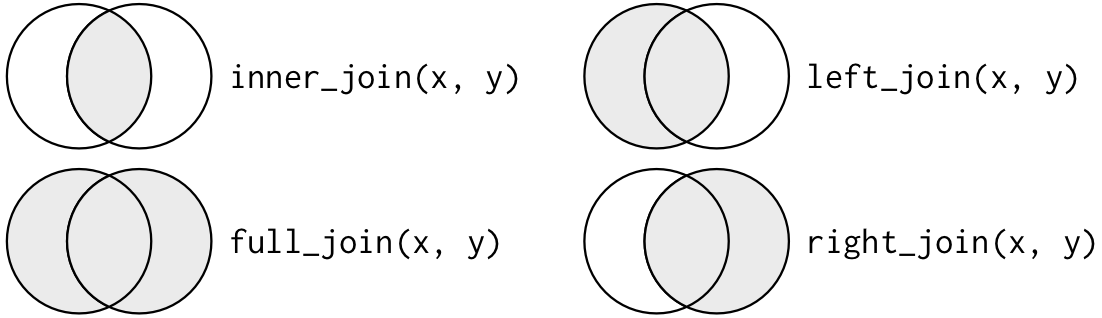
Suppose we want to create a table that combines the information about COVID-19 deaths (c19_df) with the information about the expenditure (hies_df) at each state.
First lets take c19_df and aggregate it at the state level.
We can use the left_join() function to merge the state_df and hies_df datasets.
left_join(x = state_df, y = hies_df, by =join_by(state==area))
# A tibble: 20 × 7
   state        deaths area_type income_mean expenditure_mean  gini poverty_rate
   <chr>         <int> <chr>           <int>            <int> <dbl>        <dbl>
 1 Johor          4740 state            8013             4793 0.366          3.9
 2 Kedah          2756 state            5522             3359 0.354          8.8
 3 Kelantan       1428 state            4874             3223 0.378         12.4
 4 Melaka         1213 state            7741             4955 0.383          3.9
 5 Negeri Semb…   1546 state            6707             4350 0.391          4.3
 6 Pahang         1037 state            5667             3652 0.33           4.3
 7 Perak          2164 state            5645             3564 0.377          7.3
 8 Perlis          199 state            5476             3468 0.334          3.9
 9 Perlis          199 district         5476             3468 0.334          3.9
10 Pulau Pinang   2085 state            7774             4630 0.359          1.9
11 Sabah          3211 state            5745             2792 0.397         19.5
12 Sarawak        1795 state            5959             3448 0.387          9
13 Selangor      11024 state           10827             5830 0.393          1.2
14 Terengganu      905 state            6815             4336 0.335          6.1
15 W.P. Kuala …   2861 state           13257             6913 0.35           0.2
16 W.P. Kuala …   2861 district        13257             6913 0.35           0.2
17 W.P. Labuan     159 state            8319             4097 0.333          3.1
18 W.P. Labuan     159 district         8319             4097 0.333          3.1
19 W.P. Putraj…     29 state           12840             7980 0.361          0.4
20 W.P. Putraj…     29 district        12840             7980 0.361          0.4
Note
The by argument indicates the column (or columns) that the two tables have in common. One more than one joining variable an be used for this statement
Quite obviously the join should give you the total number of rows on the left side of your statement. Note in the above case there are 20 rows because there are four districts with the same name as states.
Inner Join
The inner_join() function only retains the rows of both tables that have corresponding values. Here we can see the difference.
inner_join(x = state_df, y = hies_df, by =join_by(state==area))
# A tibble: 20 × 7
   state        deaths area_type income_mean expenditure_mean  gini poverty_rate
   <chr>         <int> <chr>           <int>            <int> <dbl>        <dbl>
 1 Johor          4740 state            8013             4793 0.366          3.9
 2 Kedah          2756 state            5522             3359 0.354          8.8
 3 Kelantan       1428 state            4874             3223 0.378         12.4
 4 Melaka         1213 state            7741             4955 0.383          3.9
 5 Negeri Semb…   1546 state            6707             4350 0.391          4.3
 6 Pahang         1037 state            5667             3652 0.33           4.3
 7 Perak          2164 state            5645             3564 0.377          7.3
 8 Perlis          199 state            5476             3468 0.334          3.9
 9 Perlis          199 district         5476             3468 0.334          3.9
10 Pulau Pinang   2085 state            7774             4630 0.359          1.9
11 Sabah          3211 state            5745             2792 0.397         19.5
12 Sarawak        1795 state            5959             3448 0.387          9
13 Selangor      11024 state           10827             5830 0.393          1.2
14 Terengganu      905 state            6815             4336 0.335          6.1
15 W.P. Kuala …   2861 state           13257             6913 0.35           0.2
16 W.P. Kuala …   2861 district        13257             6913 0.35           0.2
17 W.P. Labuan     159 state            8319             4097 0.333          3.1
18 W.P. Labuan     159 district         8319             4097 0.333          3.1
19 W.P. Putraj…     29 state           12840             7980 0.361          0.4
20 W.P. Putraj…     29 district        12840             7980 0.361          0.4
Does inner_join give different results to left_join in the above example?
Right Join
The right_join() function is like the left_join() function except that it gives priority to the “right” hand argument.
right_join(x = state_df, y = hies_df, by =join_by(state==area))
# A tibble: 998 × 7
   state        deaths area_type income_mean expenditure_mean  gini poverty_rate
   <chr>         <int> <chr>           <int>            <int> <dbl>        <dbl>
 1 Johor          4740 state            8013             4793 0.366          3.9
 2 Kedah          2756 state            5522             3359 0.354          8.8
 3 Kelantan       1428 state            4874             3223 0.378         12.4
 4 Melaka         1213 state            7741             4955 0.383          3.9
 5 Negeri Semb…   1546 state            6707             4350 0.391          4.3
 6 Pahang         1037 state            5667             3652 0.33           4.3
 7 Perak          2164 state            5645             3564 0.377          7.3
 8 Perlis          199 state            5476             3468 0.334          3.9
 9 Perlis          199 district         5476             3468 0.334          3.9
10 Pulau Pinang   2085 state            7774             4630 0.359          1.9
# ℹ 988 more rows
What about now?
Acknowledgements
Material for this lecture was borrowed and adopted from