Practical Statistics 3: Powering up! Descriptive and Inferential Statistics

COVID-19 Vaccinations and Death in Malaysia

Task 1: Descriptive statistics using tidyverse

Question: Compute the summary statistics (count, mean, standard deviation, minimum, and maximum) of age using tidyverse functions.

Steps:

  1. Install and load the tidyverse package.

  2. Filter the dataset to remove missing values in the “age” column (Note there are no missing values in the dataset- the task is simply meant to simulate the code that would be required if there were).

  3. Use the summary functions from dplyr to compute the required summary statistics. In this case- count, mean, standard deviation, minimum, and maximum

Solution:

# Step 1
#install.packages("tidyverse")
library(tidyverse)

# Step 2 & 3
summary_age <- c19_df %>% filter(!is.na(age)) %>% 
  summarise(
  count = n(),
  mean = mean(age),
  sd = sd(age),
  min = min(age),
  max = max(age)
)
summary_age
  count     mean       sd min max
1 37152 62.65464 16.58926   0 130

Task 2: Descriptive statistics using gtsummary

Question: Create a descriptive statistics table for age, male, bid, and malaysian variables using gtsummary.

Steps:

  1. Install and load the gtsummary package.

  2. Create a subset of the data with the selected variables (Note: Select any five variables).

  3. Use the tbl_summary() function to compute and display the descriptive statistics.

  4. Stratify by any other selected variable.

Solution:

# Step 1
#install.packages("gtsummary")
library(gtsummary)

# Step 2, 3 & 4
df_subset <- c19_df %>% 
  select(age, male, bid, malaysian) %>% 
  tbl_summary(by = malaysian)

Task 3: Inferential statistics using rstatix

Question: Test if there is a significant difference in age between males and females using the t-test.

Steps:

  1. Install and load the rstatix package.

  2. Filter the dataset to remove missing values in the “age” and “male” columns.

  3. Recode the “male” variable to factor.

  4. Conduct a t-test to compare the means.

Solution:

# Step 1
#install.packages("rstatix")
library(rstatix)

# Step 2
c19_df <- c19_df %>% filter(!is.na(age), !is.na(male))

# Step 3
c19_df$male <- factor(c19_df$male, levels = c(0, 1), labels = c("Female", "Male"))

# Step 4
c19_df %>% t_test(age ~ male)
# A tibble: 1 × 8
  .y.   group1 group2    n1    n2 statistic     df        p
* <chr> <chr>  <chr>  <int> <int>     <dbl>  <dbl>    <dbl>
1 age   Female Male   15783 21369      9.05 32644. 1.55e-19

Task 4: Inferential statistics using gtsummary

Question: Test if there is a significant difference in age between Malaysians and non-Malaysians using the t-test, and present the results in a table using gtsummary.

Steps:

  1. Recode the “malaysian” variable to factor (Tip: Use the factor function).

  2. Use the tbl_summary() function to present the results.

Solution:

# Step 1
c19_df$malaysian <- factor(c19_df$malaysian, levels = c(0, 1), labels = c("Non-Malaysian", "Malaysian"))

# Step 2
t_test_result <- c19_df %>% 
  select(age, malaysian) %>%                 # keep variables of interest
  tbl_summary(                               # produce summary table
    statistic = age ~ "{mean} ({sd})",       # specify what statistics to show
    by = malaysian) %>%                      # specify the grouping variable
  add_p(age ~ "t.test") 
t_test_result
Characteristic Non-Malaysian, N = 4,0341 Malaysian, N = 33,1181 p-value2
age 49 (14) 64 (16) <0.001
1 Mean (SD)
2 Welch Two Sample t-test

Task 5: Correlations using corrr

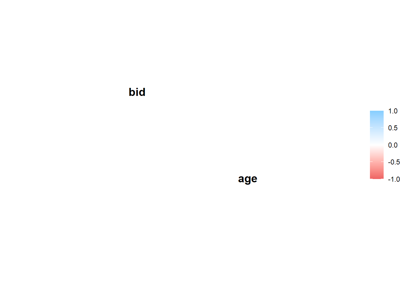
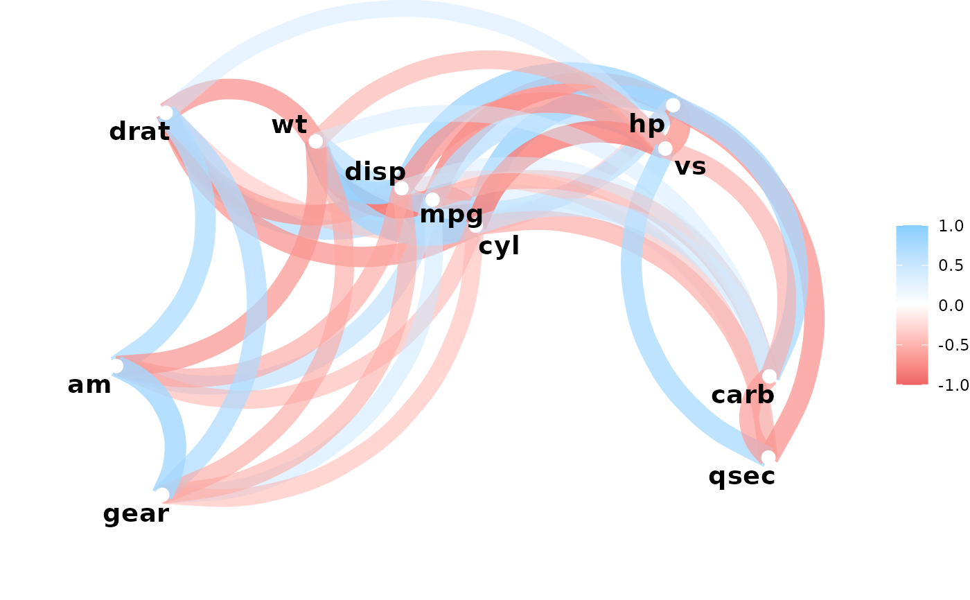
Question: Compute the correlation between age, male, bid, and malaysian variables, and represent it in a correlation plot (Note: The selection of categorical variables is by design- just to practice the selection and presentation)

Steps:

  1. Install and load the corrr package.

  2. Create a subset of the data with the selected variables.

  3. Compute the correlation matrix (Note: Try ?network_plot and see how this can be used)

# Step 1
#install.packages("corrr")
library(corrr)

# Step 2
df_subset <- c19_df %>% select(age, male, bid, malaysian)

# Step 3
correlation_matrix <- df_subset %>% correlate()
Non-numeric variables removed from input: `male`, and `malaysian`
Correlation computed with
• Method: 'pearson'
• Missing treated using: 'pairwise.complete.obs'
# Step 4
correlation_matrix %>% network_plot()

This would be the outcome if anything was highly correlated in our data.